Cable Life Prediction: From Test Cycles to Real Maintenance Intervals
Quick Answer: A flex test number becomes a service life only after conversion: duty per cycle, acceleration factors, a safety margin and a wear-out model stand between twenty million test cycles and a maintenance interval your planner can schedule.
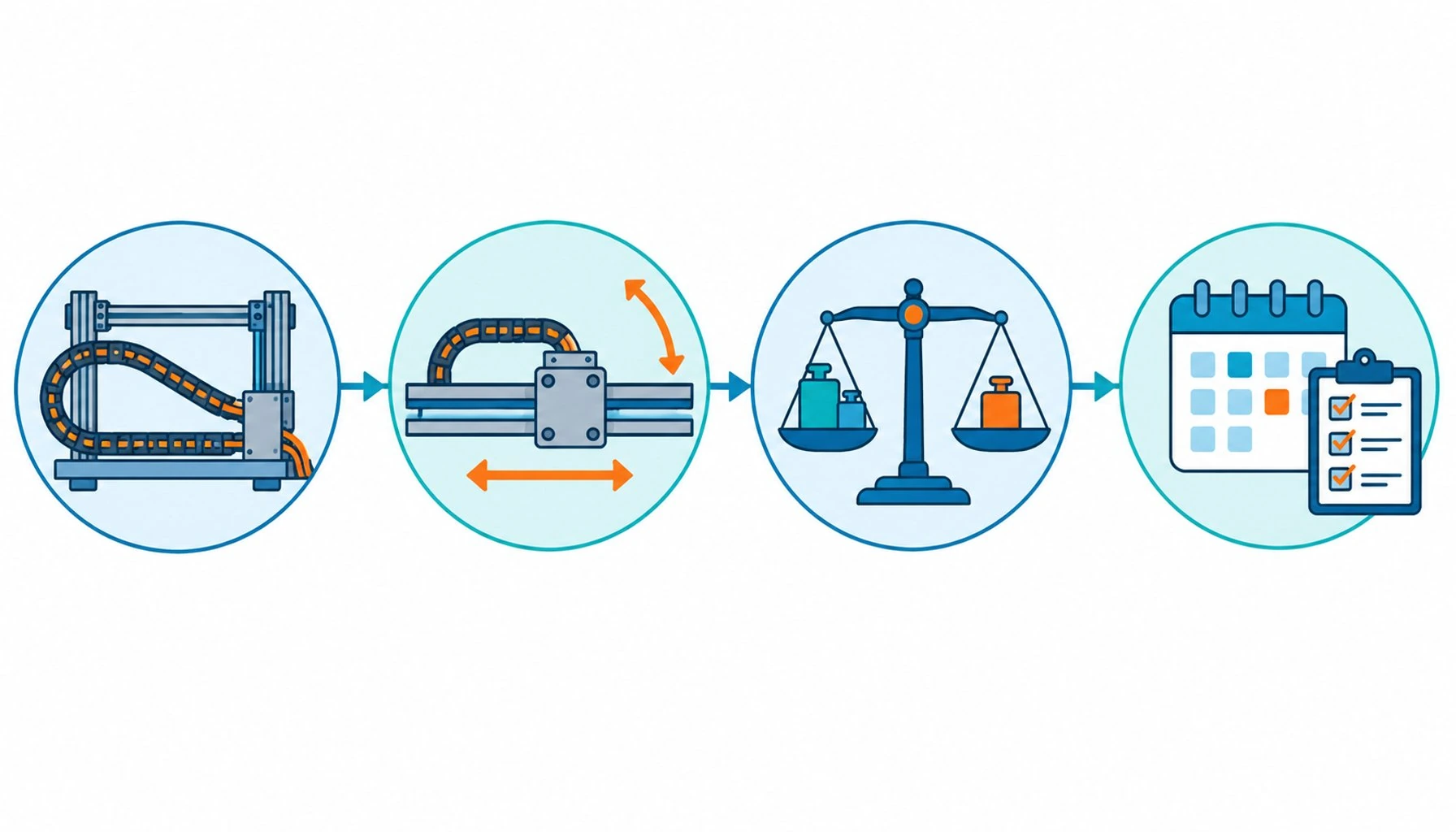
Cable life prediction is where laboratory evidence finally earns its keep, or fails to. Every buyer has seen the cycle number; fewer have seen the arithmetic that turns it into “inspect at month nine, replace in the next shutdown.” The conversion is not mysterious, but it has steps, and skipping steps is how cables get replaced either embarrassingly early, at warranty prices, or dramatically late, at downtime prices. This guide walks the path from test rig to maintenance plan: how duty and test conditions compare, what acceleration and safety factors contribute, how scatter changes the question from when a cable fails to when a fleet of cables starts failing, and how the resulting estimate lands in a maintenance schedule where condition checks keep it honest.
Introduction
The starting point is an honest frame: cable life prediction is estimation with error bars, not prophecy. A moving cable fails through fatigue, and fatigue scatters, two nominally identical cables on identical axes can differ substantially in life. What prediction can do is place the failure zone on a calendar with useful confidence, enough to plan inspection and replacement before downtime plans for you. What it cannot do is name the week. Buyers and maintenance planners who accept the error bars get schedules that work; those who expect certainty get disappointed by mathematics that was never on the quotation.
The evidence the prediction consumes comes from the test layer: rig type, radius, speed, load and failure definition, the five parameters covered in the flex testing guide’s logic. This guide assumes those inputs exist and asks what happens next.
Step One: Convert the Test Into Duty
The first arithmetic is dimensional. A test number counts cycles at defined conditions; the machine runs cycles of its own shape. Compare them per unit: cycles per shift on the axis against cycles per test unit at the same radius and speed, and the ratio gives the first conversion factor. If the application’s radius matches the test’s, the transfer is direct; if the application bends tighter, the conversion is not linear, because fatigue life falls steeply with radius, and an honest estimate applies the steepness rather than pretending proportionality. Speed differences work similarly, faster cycles are harder cycles, and load differences add their own factor where the test ran light and the machine runs heavy.
At the end of step one you have a number of machine-cycles the test evidence supports, stated at your duty rather than the rig’s. It is an estimate, and it is already more useful than the raw datasheet figure, which describes a duty your machine does not run.
Step Two: Apply the Factors That Machines Add
Real installations subtract life in ways the rig does not model, and the prediction must pay for them. Installation quality is first: a cable clamped at the wrong point or run at a radius transition spends its margin early. Environment is second: oil exposure, abrasion at edges and temperature extremes each take a bite, and the bites compound. Scatter is third: the estimate should aim at the failure of a population, not of the luckiest sample, which is where statistical thinking earns its place, treating observed test scatter as a spread rather than a point.
The response is the safety factor, a deliberate haircut applied to the converted number. The size of the haircut reflects how well the duty is known: a stable, measured duty on a well-matched cable supports a modest margin; a duty with unknowns, variable payloads, harsher chemistry than documented, supports a larger one. Safety factors are not cowardice; they are the price of the difference between a test and a machine, and planners who skip them buy their cables back with downtime interest. The failure sources the haircut pays for are cataloged in the guide to common cable failure causes.
| Input | What it contributes | Where it comes from | Typical mistake |
|---|---|---|---|
| Test conditions | The duty the evidence actually covers | Supplier test report: rig, radius, speed, load, end point | Treating the headline cycles as duty-independent |
| Application duty | Cycles per shift at the real radius and speed | Motion profile and shift plan | Using design duty after the machine's use has grown |
| Radius and speed correction | Non-linear adjustment when duty differs from test | Fatigue behavior of the construction class | Assuming life scales linearly with radius |
| Environment deductions | Life spent on oil, abrasion and temperature | Route survey and fluid inventory | Adding environment as an afterthought |
| Scatter and safety factor | Population failure behavior, not luckiest sample | Test batch spread and duty uncertainty | Planning to the average and being early half the time |
Step Three: From Estimate to Maintenance Plan
The life estimate becomes a plan through two schedules. The inspection schedule rides ahead of the estimate: visual checks of the bend zone, jacket and terminations at intervals that catch the wear before it finishes, quarterly at first, tuned by what the checks find. The replacement schedule rides on the estimate: the cable is due for replacement in a planned window before the predicted failure zone, not after the first fault. The two work as a pair, the estimate sets the calendar, and the inspections correct it; a cable inspected at month six and found pristine supports a longer interval next cycle, and one showing jacket wear early moves its replacement forward. Condition evidence, continuity checks and insulation measurements, sharpens the picture further, and the acceptance-test logic behind such evidence is treated in the guide to factory acceptance testing.
The plan’s shape for a fleet matters as much as for a single axis: machines run their axes unequally, and identical cables age at different rates. Tracking per axis, with replacement windows staggered by actual duty, turns cable replacement from an emergency response into a routine line on the shutdown plan.
| Decision | Basis | Trigger to adjust |
|---|---|---|
| Inspection interval | Lead time ahead of the predicted wear zone | Findings at checks, clean supports longer, wear shortens |
| Replacement window | Predicted life minus safety factor, on the shutdown plan | Inspection findings or duty changes since commissioning |
| Per-axis stagger | Actual cycle counts per axis, not fleet averages | Production pattern shifts between axes |
| Spare holding | Population behavior around the predicted window | Earlier-than-expected first failures in the fleet |
| Root-cause review | Every early failure examined against the prediction | A pattern, routing, environment or construction, shows up |
When Prediction Is Not the Answer
Honest limits: prediction inherits every weakness of its inputs, and some duties lack the inputs altogether. Non-standard motion, combined torsion and tight radius, has thin test data behind it; environments with unquantified chemistry resist the correction factors; and retrofit installations with unknown histories start from guesswork. In these territories the honest plan shifts weight from prediction to inspection, shorter intervals, closer watching, and treats the first replacement as data collection for the second estimate. Prediction also stops at the cable: connectors, glands and fixings age on their own schedules and fail their own ways, and a maintenance plan that watches only the cable watches half the system. The supplier vetting questions that establish how much evidence a prediction can lean on are covered in the guide to vetting equipment manufacturers.
RFQ Checklist: Evidence to Request for Life Prediction
Attach these items to the RFQ so the arithmetic starts on solid ground:
- Test reports with all five parameters stated: rig, radius, speed, load, failure end point
- Batch-based results with scatter, not single-sample best cases
- Application duty statement from your side: cycles per shift, radii, speeds, environment
- Supplier position on radius and speed corrections when duty differs from test
- Wear indicators: what early damage looks like on this construction, and where to look
- Support for a pilot interval: supplier agreement to review inspection findings at the first window
The reading discipline that keeps all of these documents honest is covered in the guide to reading equipment datasheets, and life prediction is the payoff of that habit.
Conclusion
Cable life prediction is a conversion, not a revelation: test cycles become duty-matched evidence, the evidence pays for the machine’s corrections, a safety factor prices the uncertainty, and the result lands on the maintenance calendar where inspections keep it honest. Buyers and planners who run the arithmetic get cable programs that cost what they planned; those who trust headline numbers get the arithmetic anyway, invoiced in downtime.
Kexingyu Cable Group (KXYE) supplies motion cable with the test evidence life prediction needs, conditions stated, scatter shown, wear indicators explained. Send your duty profile through the RFQ page, and we will quote the cable and the arithmetic together.